Pretty Brownian motion simulations
As I went through a laptop upgrade and migration recently, I discovered remnants of my old academic webpage. I found this post which has some pretty diagrams for simulations of Brownian motion and related mathematical objects. I thought it could be interesting to reproduce so that these pretty diagrams don’t get lost forever! Incidentally, I really enjoyed learning about Brownian motion, and I revisit my lecture notes from time to time.
In this page, you will find a few small simulations I ran about Brownian motion and related processes. I just think it looks cool. Don’t expect any kind of real explanation of what is going on. I learned most of what I know about Brownian motion from Louigi Addario-Berry’s Fall 2016 course on Brownian motion, largely based on the free book by Peter Mörters, and Yuval Peres.
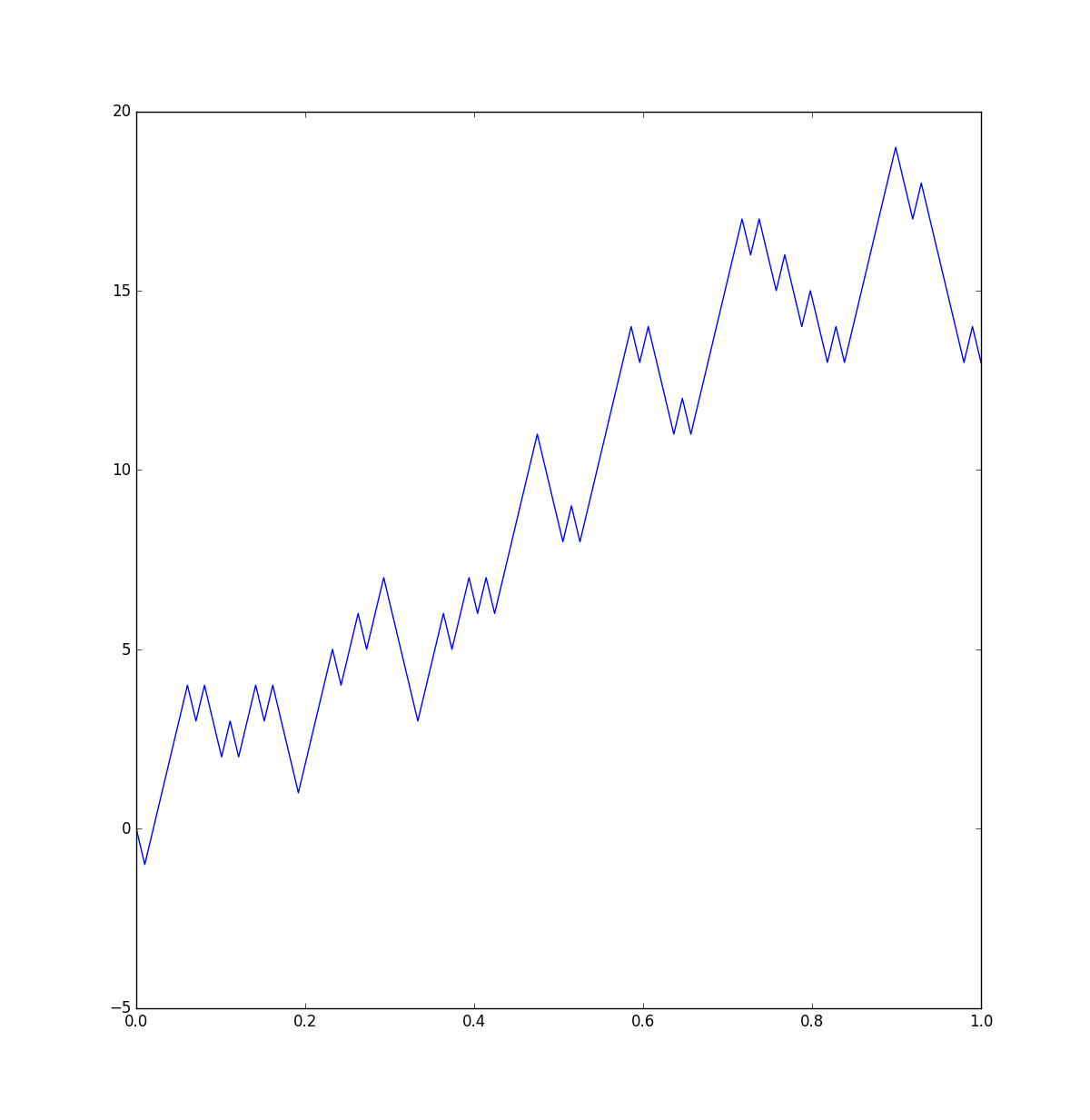
It is very easy to algorithmically generate a Brownian motion to any desired degree of precision via Lévy’s construction. Alternatively, one can approximate Brownian motion by scaling a simple random walk, i.e., a uniform random walk starting from 0, which steps upwards or downwards with equal probability, scaled appropriately. The central limit theorem suggests that the correct scaling factor should be \(1/\sqrt{n}\). See, first, a simple random walk on a few steps, not rescaled:
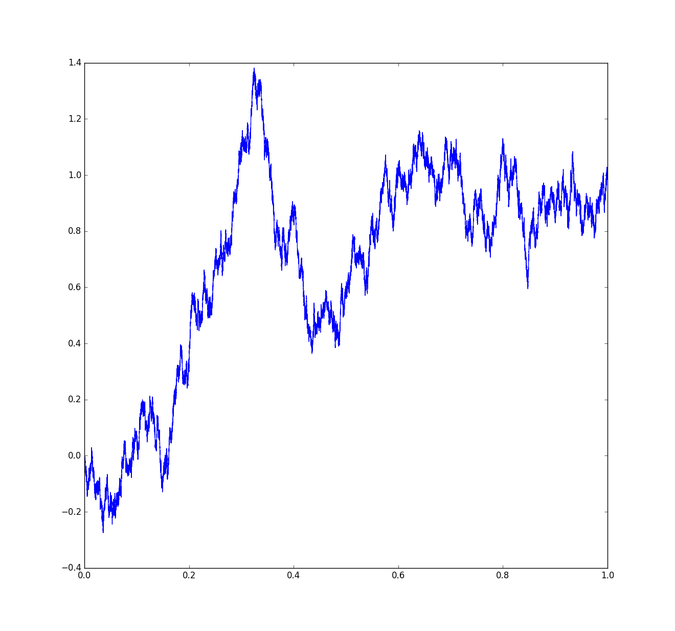
Now, after rescaling appropriately, it starts to look like Brownian motion:
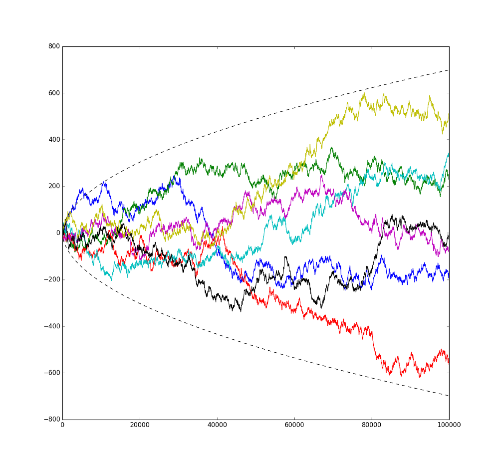
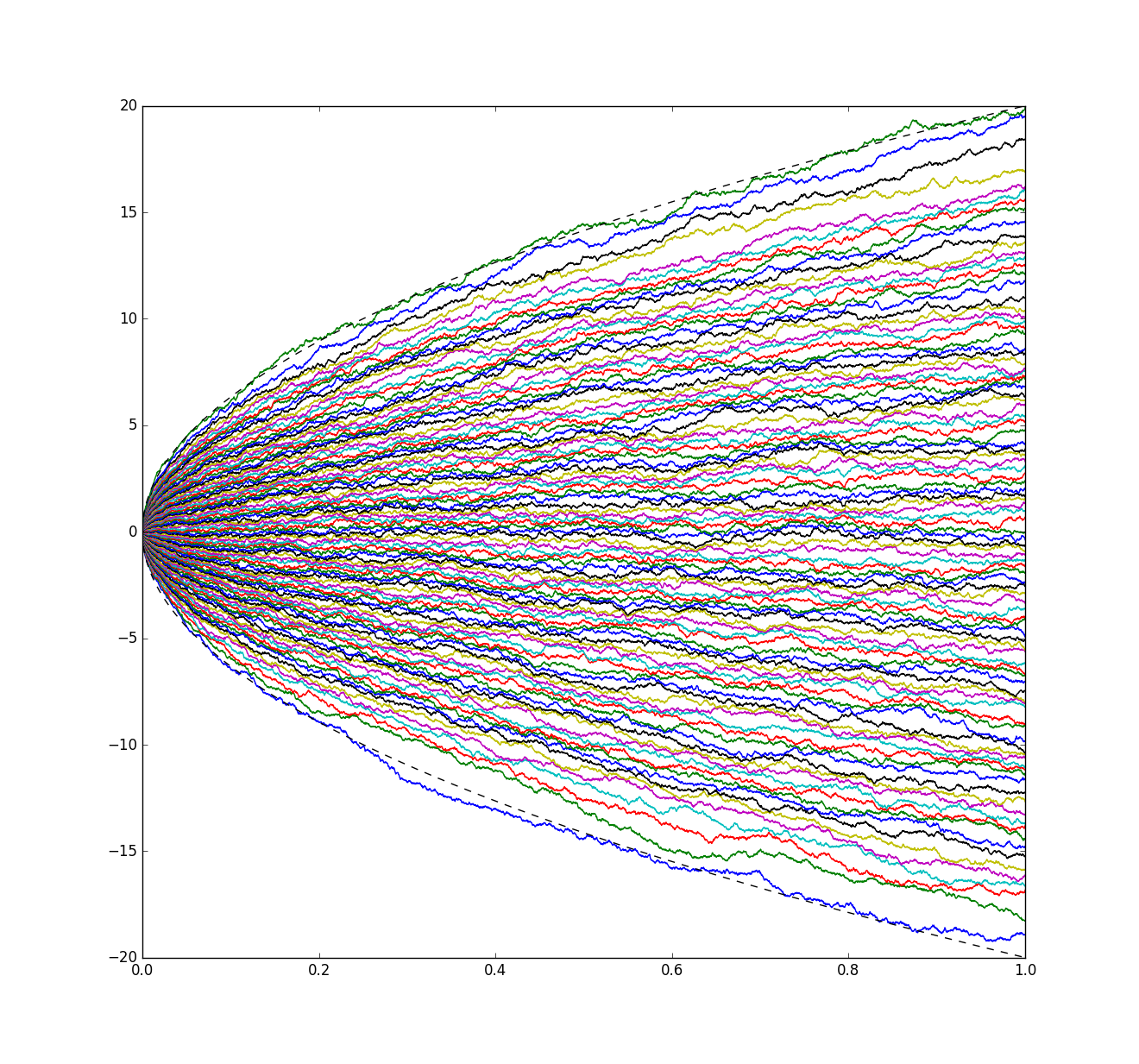
In the following, you can see a few independent Brownian motions, including the upper and lower envelopes at \(\sqrt{2t \log \log t}\), which are known to almost surely tightly bound the trajectory of Brownian motion:
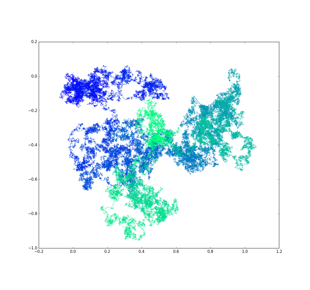
And now, a planar Brownian motion. Cool:
One can also look at a symmetric matrix whose entries form independent Brownian motions. The induced walk on the eigenvalues of such a matrix is called the Dyson-Brownian motion. The empirical distribution of eigenvalues converges to the Wigner semicircle distribution. I generated a Dyson-Brownian motion on a 100x100 matrix, also plotting the upper and lower envelopes at \(2\sqrt{n}\), bounding the largest eigenvalue in absolute value:
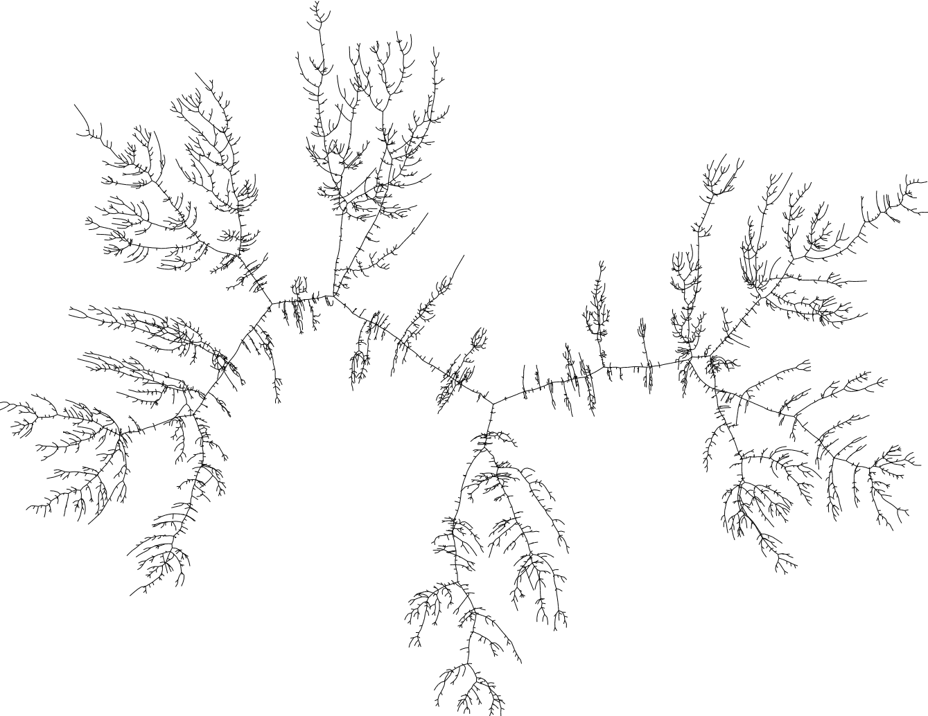
There is also Brownian-kind of tree, called the Brownian Continuum Random Tree (CRT). First note that we can encode a rooted plane tree by a walk by tracing its contour in a depth-first search; this is actually a bijection. Hence, once can expect a random “continuous” tree to arise by decoding a Brownian excursion in the above sense. In fact, Aldous described this object and showed that it is a scaling limit of a uniformly random Cayley tree. Cayley trees are very easy to generate (actually, in linear time), via the correspondence with Prüfer codes. I generated a uniformly random Cayley tree on 10000 nodes to give a good idea of what the Brownian CRT should (structurally) look like. The graph was drawn using Graphviz: